Kolmogorov Module
The Kolmogorov module houses code that deals with the stationary distribution of a model, named for the Kolmogorov forward equations (Fokker-Planck) which form the basis for calculation of the stationary distribution. For details on calculation methods, please see Markus Brunnermeier’s ECON 529 course. As of December 2021, the stationary distribution calculation notes were in Chapter 3, and the notes were publicly available from the linked website.
-
PyMacroFin.kolmogorov.stationary_distribution(state, mu, sig, plot=True, t=[], init=[], return_mesh=False)¶ Estimate stationary distribution given a state grid with drift and volatility. This function uses the basis of the adjoint of the Kolmogorov Forward / Fokker-Planck operator as described in Chapter 3 of Markus Brunnermeier and Yuily Sannikov’s ECON 529 Notes (see here).
Parameters: - state: pd.core.series.Series or pd.core.frame.DataFrame
Vector or matrix of state variable values. If the problem is one-dimensional,
stateshould be a named series with the name being the name of the state variable. If the problem is two-dimensional,stateshould be a DataFrame with two columns, named for the two state variables. The DataFrame should contain a row for each combination of values to be used in the discretization of the state space.- mu: pd.core.series.Series of pd.core.frame.DataFrame
Vector or matrix of drifts corresponding to the brownian motion of the state variable(s) at the discrete points of
state. If the problem is one-dimensional, this should be a single vector (series). If the problem is two-dimensional, this should be a DataFrame with columns names matching the column names instate. The column corresponding to a state variable should contain the drifts in that state variable direction. There should not be drifts leading outside the grid (i.e.mu.iloc[0]>=0andmu.iloc[-1]<=0in the 1D case).- sig: pd.core.series.Series of pd.core.frame.DataFrame
Vector or matrix of volatilities corresponding to the brownian motion of state variable(s) at the discrete points of
state. If the problem is one-dimensional, this should be a single vector (series). If the problem is two-dimensional, this should be a DataFrame with columns names matching the column names instate, as well as a column named'cross'. The column corresponding to a state variable should contain the volatility (standard deviation) of that state variable direction, and the'cross'column should contain the cross volatility term (again in standard deviation form). The first and last volatilities should be zero in the grid (i.e.sig.iloc[0]=0and sig.iloc[-1]=0 in the 1D case).- plot: bool
Whether or not to plot the distribution. Defaults to
True- return_mesh: bool
Whether or not to return a mesh object for use with the
stationary_plot_2dfunction. If generating thepdfsreturn object, returning the mesh is useful to plot the distribution from any given time point. If the problem is one-dimensional, this argument has no effect.
Returns: - pdf: pd.core.frame.DataFrame
Estimated stationary distribution
Notes
- There should be no NaN or inf in the input vectors / matrices. NaNs or infs will cause undesired behavior.
- If the function fails, you may try running wtih a
tvector to see how the distribution evolves from an initial known distribution. It may be the case that your stationary distribution is degenerate. - Note that this function will fail in most instances if the volatility at grid boundaries is nonzero and if drifts point toward outside the grid at or near boundaries.
-
PyMacroFin.kolmogorov.stationary_distribution_model(m, df, plot=True, t=[], init=[], return_mesh=False)¶ Estimate stationary distribution given a PyMacroFin model object and solution DataFrame. This function uses the basis of the adjoint of the Kolmogorov Forward / Fokker-Planck operator as described in Chapter 3 of Markus Brunnermeier and Yuily Sannikov’s ECON 529 Notes (see here).
Parameters: - m: PyMacroFin.model.macro_model
Model object to which the solution belongs
- df: pd.core.frame.DataFrame
DataFrame returned by
df = m.run()with the optionm.options.return_solution = True.- t: iterable
Vector of times.
- init: pd.core.series.Series
Vector the same size first dimension as
dfbeing the initial distribution (starting point) for iterating forward in time iftis nonempty.- return_mesh: bool
Whether or not to return a mesh object for use with the
stationary_plot_2dfunction. If generating thepdfsreturn object, returning the mesh is useful to plot the distribution from any given time point. If the problem is one-dimensional, this argument has no effect.
Returns: - pdf: np.array
Estimated stationary distribution
- pdfs: np.array
This object is only returned when
tis nonempty. If the problem is one-dimensional, this returns a two-dimensional array with the second dimension corresponding to the entries int. Hence,pdfswill contain the distribution vector for each time int.
Notes
- If the function fails, you may try running wtih a
tvector to see how the distribution evolves from an initial known distribution. It may be the case that your stationary distribution is degenerate. - Note that this function will fail in most instances if the volatility at grid boundaries is nonzero and if drifts point toward outside the grid at or near boundaries.
-
PyMacroFin.kolmogorov.stationary_plot_1d(pdf, state, name, save=False)¶ Plot the stationary distribution for a one-dimensional problem
Parameters: - pdf: np.array
The distribution vector to be plotted
- state: np.array
The state variable vector corresponding to the values in
pdf- name: str
The name of the state variable.
- save: False or str
If
Falsethen the plot is not saved. If a string, then the string passed must be a valid path to which to save the file.
Returns: - Null. The distribution is plotted (and saved if specified).
-
PyMacroFin.kolmogorov.stationary_plot_2d(pdf, mesh, save=False, engine='mpl', view=(30, - 60))¶ Plot the stationary distribution for a two-dimensional problem
Parameters: - pdf: np.array
The two-dimensional distribution grid to be plotted.
- mesh: tuple
This argument must be a tuple with four entries. The first two entries must be the two-dimensional mesh corresponding to the state-space of the distribution. For example, if the distribution is over a 50x50 grid of variables x and y, where x and y are both length 50 vectors, then running
xx, yy = numpy.meshgrid(x,y)will produce the first two entries of mesh. The second two entries of mesh are the names of the two state variables.- save: False or str
If
Falsethen the plot is not saved. If a string, then the string passed must be a valid path to which to save the file.- engine: str
Whether to use
matplotlib(engine='mpl') orplotly(engine='plotly'). Defaults to'mpl'.- angle: numeric
Tuple of elevation and azimuth angles from which to view the plot. This argument is only used for the
'mpl'engine.
Returns: - Null. The distribution is plotted (and saved if specified).
Examples
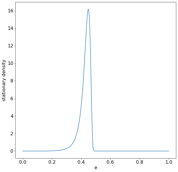
A verifiable test case using the stationary distribution function in PyMacroFin is the case of the model used in Chapter 3 of Professor Brunnermeier’s ECON 529 Notes. Obtaining the drifts and volatilities from either the Matlab code available in the notes or by using PyMacroFin, you may run
pdf = stationary_distribution(eta,mu,sig,plot=True)
which results in the following plot: